Real-time motor imagery decoding with CSP

Adapts MNE’s Motor imagery decoding from EEG data using the Common Spatial Pattern (CSP) tutorial to MNE-RT’s real-time architecture, using the PhysioNet EEG Motor Movement/Imagery Dataset:

1. Load left- vs. right-hand imagery epochs (runs 6, 10, 14, subject 1).

2. Fit RTDecode (CSP + logistic regression) on most of the epochs, holding a few epochs per class out for the live demo below.

3. Cross-validate the offline classification accuracy and plot the learned CSP spatial patterns — exactly the core content of the MNE tutorial above.

4. Concatenate the held-out epochs into one continuous array (known, deterministic left/right timeline) and stream it through connect_to_array() — no LSL networking required.

5. Attach the fitted decoder via set_decoder() and run record_main() with modality=["decode"]: the classifier is queried once per acquisition window, live, exactly as it would be during a real closed-loop BCI session.

6. Plot the live decoded probability trace against the true left/right timeline to confirm the real-time classifier tracks it.

Note

This is a small, single-subject demo (45 trials total) meant to show the real-time decoding mechanics working end-to-end — not a benchmark of CSP decoding accuracy. Expect modest offline accuracy; see MNE’s tutorial for a fuller discussion of CSP decoding performance.

Note

Downloads ~15 MB of data on first run via mne.datasets.eegbci.load_data().

Load PhysioNet EEGBCI motor imagery data

import tempfile
from pathlib import Path

import matplotlib.pyplot as plt
import mne
import numpy as np
from sklearn.model_selection import ShuffleSplit, cross_val_score

from mne_rt import RTDecode, RTStream

mne.set_log_level("WARNING")

SUBJECT = 1
RUNS = [6, 10, 14]
files = mne.datasets.eegbci.load_data(SUBJECT, RUNS, update_path=True, verbose=False)
raws = [mne.io.read_raw_edf(f, preload=True, verbose=False) for f in files]
raw = mne.concatenate_raws(raws)
mne.datasets.eegbci.standardize(raw)
raw.set_montage(mne.channels.make_standard_montage("standard_1005"), on_missing="ignore")
raw.filter(l_freq=1.0, h_freq=40.0, verbose=False)

SFREQ = raw.info["sfreq"]
print(f"Channels: {raw.info['nchan']}  |  sfreq: {SFREQ:.0f} Hz")

/home/runner/work/mne-rt/mne-rt/examples/ex_motor_imagery_decode.py:60: FutureWarning: Montage name 'standard_1005' is deprecated and will be removed in MNE 1.14. Use 'colin27_1005' instead.
  raw.set_montage(mne.channels.make_standard_montage("standard_1005"), on_missing="ignore")
Channels: 64  |  sfreq: 160 Hz

Extract fixed-length imagery epochs

Unlike NF feature extraction (which can use any window length), a decoder must be fit and queried on windows of the same duration — here 2 s, starting 1 s after the imagery cue to avoid the cue-onset transient. This duration must later match record_main’s winsize.

events, event_id = mne.events_from_annotations(raw, verbose=False)
WINSIZE = 2.0
TMIN = 1.0
TMAX = TMIN + WINSIZE

epochs = mne.Epochs(
    raw,
    events,
    event_id={"left": event_id["T1"], "right": event_id["T2"]},
    tmin=TMIN,
    tmax=TMAX,
    baseline=None,
    preload=True,
    verbose=False,
)
print(f"Epochs: {len(epochs)}  |  left={len(epochs['left'])}  right={len(epochs['right'])}")

Epochs: 45  |  left=21  right=24

Hold out epochs for the live streaming demo

A few epochs per class are set aside now, before fitting, and streamed live further down — the decoder never sees them during calibration.

N_TEST_PER_CLASS = 8
train_idx, test_idx = [], []
for label in ("left", "right"):
    idx = np.where(epochs.events[:, 2] == epochs.event_id[label])[0]
    test_idx.extend(idx[:N_TEST_PER_CLASS])
    train_idx.extend(idx[N_TEST_PER_CLASS:])
epochs_train = epochs[sorted(train_idx)]
epochs_test = epochs[sorted(test_idx)]

X_train = epochs_train.get_data()
y_train = np.where(epochs_train.events[:, 2] == epochs.event_id["left"], "left", "right")

Fit RTDecode and cross-validate offline

RTDecode assembles the exact CSP + classifier sklearn.pipeline.Pipeline from the MNE tutorial internally (decoder.pipeline), so it plugs directly into sklearn.model_selection.cross_val_score for offline validation.

decoder = RTDecode(info=epochs.info, spatial_filter="csp", n_components=4)

cv = ShuffleSplit(n_splits=5, test_size=0.2, random_state=0)
scores = cross_val_score(decoder.pipeline, X_train, y_train, cv=cv, n_jobs=1)
print(f"Cross-validated accuracy: {scores.mean():.2f} +/- {scores.std():.2f}  (chance = 0.50)")

decoder.fit(X_train, y_train, verbose=False)

Cross-validated accuracy: 0.47 +/- 0.12  (chance = 0.50)

<RTDecode | spatial_filter='csp', estimator=LogisticRegression, fitted>

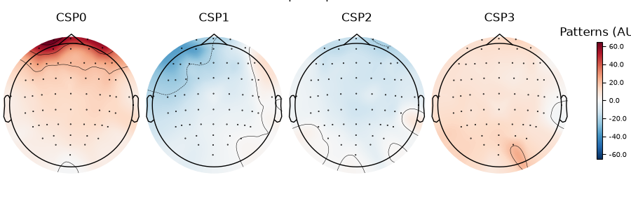
Figure 1 — CSP spatial patterns

The most discriminative spatial filters typically localise over sensorimotor cortex (around C3/C4), matching the MNE tutorial’s figure.

csp = decoder.pipeline.named_steps["csp"]
fig1 = csp.plot_patterns(
    epochs.info,
    components=range(csp.n_components),
    ch_type="eeg",
    units="Patterns (AU)",
    size=1.5,
)
fig1.suptitle("CSP spatial patterns", y=1.05)

Text(0.5, 1.05, 'CSP spatial patterns')

Real-time decoding via connect_to_array

The held-out test epochs are concatenated, in order, into one continuous array — this gives an exactly-known left/right timeline to validate the live decoder against, with no LSL networking or recorded file required (see connect_to_array()).

test_data = epochs_test.get_data()
test_labels = np.where(epochs_test.events[:, 2] == epochs.event_id["left"], "left", "right")
stream_data = np.concatenate(list(test_data), axis=1)
n_samples_per_segment = test_data.shape[2]

tmp_dir = Path(tempfile.mkdtemp(prefix="mne_rt_decode_demo_"))

nf = RTStream(
    subject_id="decode01",
    session="01",
    subjects_dir=str(tmp_dir),
    montage=None,
    data_type="eeg",
    verbose=False,
)
nf.connect_to_array(stream_data, epochs.info, chunk_size=16, n_repeat=1)
nf.set_decoder(decoder)

duration = stream_data.shape[1] / SFREQ
nf.record_main(
    duration=duration,
    modality=["decode"],
    winsize=WINSIZE,
    show_nf_signal=False,
    show_raw_signal=False,
    show_topo=False,
    save_raw=False,
    verbose=False,
)

proba = np.asarray(nf.nf_data["decode"])
hop_s = WINSIZE * 0.5  # record_main uses 50% window overlap

n_correct = 0
for i, label in enumerate(test_labels):
    t0, t1 = i * n_samples_per_segment / SFREQ, (i + 1) * n_samples_per_segment / SFREQ
    seg = proba[int(t0 / hop_s) : int(t1 / hop_s)]
    predicted = "right" if seg.mean() >= 0.5 else "left"
    n_correct += predicted == label

print(
    f"Live segment-level accuracy: {n_correct}/{len(test_labels)} "
    f"({100 * n_correct / len(test_labels):.0f} %)"
)

Live segment-level accuracy: 9/16 (56 %)

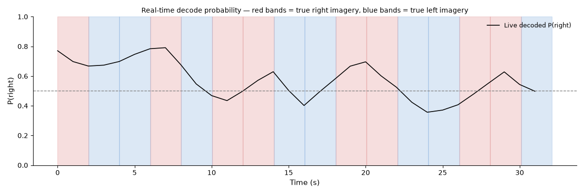
Figure 2 — live decoded probability vs. the true timeline

Grey/white bands mark the true left/right segments in the streamed test data; the trace is RTDecode’s live P(right) for each acquisition window, queried in real time by record_main().

t = np.arange(len(proba)) * hop_s

fig2, ax = plt.subplots(figsize=(12, 4))
for i, label in enumerate(test_labels):
    t0 = i * n_samples_per_segment / SFREQ
    t1 = (i + 1) * n_samples_per_segment / SFREQ
    ax.axvspan(t0, t1, alpha=0.15, color="#C62828" if label == "right" else "#1565C0")
ax.plot(t, proba, color="black", lw=1.2, label="Live decoded P(right)")
ax.axhline(0.5, color="grey", ls="--", lw=1.0)
ax.set_xlabel("Time (s)", fontsize=11)
ax.set_ylabel("P(right)", fontsize=11)
ax.set_title(
    "Real-time decode probability — red bands = true right imagery, blue bands = true left imagery",
    fontsize=10,
)
ax.set_ylim(0, 1)
ax.legend(fontsize=9, frameon=False, loc="upper right")
ax.spines[["top", "right"]].set_visible(False)
fig2.tight_layout()