User Guide#

This page introduces the core concepts behind real-time M/EEG processing and explains how MNE-RT maps those concepts onto a concrete session workflow. No prior BCI or neurofeedback experience is required.

Real-time M/EEG processing #

Real-time M/EEG processing refers to any pipeline that acquires brain signals, extracts features as fast as the data arrives, and delivers results — feedback, monitoring outputs, or triggers — within a latency budget of milliseconds to seconds. MNE-RT covers the full range: continuous neurofeedback, event-related ERP/TFR analysis, BCI decoding, and passive brain monitoring.

① Brain signal

EEG or MEG electrodes pick up cortical oscillations from the scalp surface in real time.

② Feature extraction

A signal processing pipeline distils the raw signal into one number per window — e.g., alpha power, laterality, or source connectivity.

③ Feedback

The feature value drives a visual, auditory, or haptic output signal — or is streamed for offline analysis or BCI control.

↑ The loop closes when the participant's self-regulation attempt changes the brain signal, which in turn changes the feedback — enabling operant conditioning of cortical activity.

Clinical applications include ADHD (theta/beta training), chronic tinnitus (auditory cortex and thalamo-cortical desynchronisation), post-stroke motor rehabilitation (sensorimotor rhythm training), and depression (frontal alpha asymmetry training).

MNE-RT Session Workflow #

Every session follows the same three-phase structure:

① Acquisition

Connect to an EEG/MEG amplifier (or mock replay) via LSL. RTStream.connect_to_lsl()

② Baseline

Record 2–5 min of resting-state data, automatically detects bad channels and computes noise covariance. Source-space work needs a head model too; that is built the first time something asks for it, so a sensor-space session never pays for it. RTStream.record_baseline()

③ Real-time

Run the closed-loop feedback loop for the prescribed duration. Feature values, reward signals, and quality metrics are streamed live and saved to BIDS. RTStream.record_main()

Phase 2 (baseline) is optional for sensor-space modalities but required for source-space modalities (it provides the noise covariance used to build the inverse operator) and for ERD/ERS-based modalities (it provides the reference power).

Closed-Loop Architecture #

The diagram below shows how data flows inside MNE-RT during a processing window:

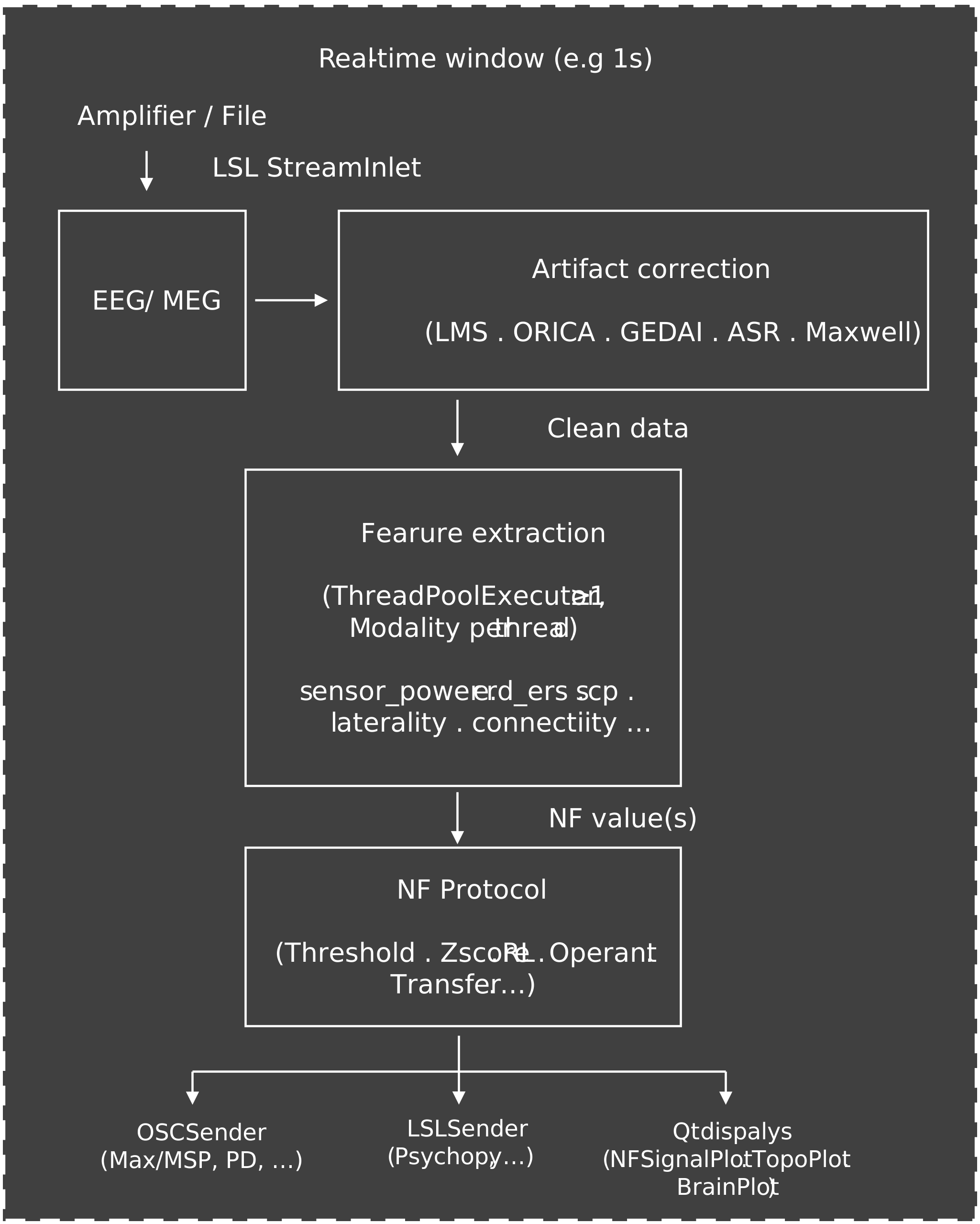
All modality computations run in a concurrent.futures.ThreadPoolExecutor, so slow operations (e.g. source-space inverse) never block the feedback display.

Key Concepts #

Feature Modality #

A modality is the brain feature that is being fed back to the participant. MNE-RT implements 20 modalities across sensor space, connectivity, and source space. You select one or more per session:

Category	Modalities	Typical use case
Sensor power	sensor_power · band_ratio · erd_ers · laterality · laterality_erd_ers	Alpha, SMR, or theta training; motor imagery
Time-domain	hjorth · entropy · scp · instantaneous_phase	SCP biofeedback; phase-triggered stimulation
Spectral peak	spectral_centroid · argmax_freq · peak_alpha_freq	Individual alpha frequency tracking
Connectivity	sensor_connectivity · connectivity_ratio · cfc_sensor · sensor_graph	Inter-hemispheric or thalamocortical coupling
Source space	source_power · source_connectivity · source_graph	Region-specific analysis; tinnitus, depression

See Real-time Feature Modalities for the mathematical definition of each.

Feedback Protocol #

A protocol decides when to deliver a reward and how much. It sits between the raw modality value and the feedback display. MNE-RT ships ten protocols:

feature value  ──▶  Protocol  ──▶  (crossed: bool, magnitude: float)
                 │
                 ├── ThresholdProtocol   fixed or slowly-adapting threshold
                 ├── ZScoreProtocol      running z-score; self-calibrating
                 ├── PercentileProtocol  tracks own rolling distribution
                 ├── LinearTrendProtocol rewards sustained directional change
                 ├── RLProtocol          ε-greedy; finds threshold automatically
                 ├── TransferProtocol    seeded from a prior session file
                 ├── OperantProtocol     FR / VR / FI / VI reward schedules
                 ├── ShamProtocol        double-blind sham wrapper
                 ├── UpDownStaircaseProtocol  converges to target success rate
                 └── MultiBandProtocol   two-band AND / OR logic

See NF Protocols for formulas and selection guidance.

Feature Combiner #

A feature combiner reduces N parallel feature values to a single mixed score. This is useful when several modalities capture complementary aspects of the brain state and you want one unified number for the protocol and display. MNE-RT provides four combiners in mne_rt.combiners:

Class	Strategy
`WeightedSumCombiner`	Normalised weighted sum `Σ(wᵢ·xᵢ)/Σ(wᵢ)`. Intuitive, interpretable. Negative weights allowed (e.g. subtract theta from alpha).
`GeometricMeanCombiner`	Weighted geometric mean `exp(Σ wᵢ·log(xᵢ)/Σwᵢ)`. Best for positive ratio or power features whose effects are multiplicative.
`ZScoredNormCombiner`	Z-score each feature against a warmup baseline, then take the Euclidean norm divided by `√n`. Returns a unit-free “deviation from baseline” score regardless of feature units or dynamic range.
`LearnedCombiner`	Pass the feature vector to any fitted `sklearn`-compatible estimator (e.g. `Ridge`, `PLSRegression`). Requires an offline calibration step but can capture non-linear feature interactions.

Example — blend alpha power and interhemispheric laterality:

from mne_rt.combiners import WeightedSumCombiner

combiner = WeightedSumCombiner(
    weights={"sensor_power": 0.6, "laterality": 0.4}
)
# Call once per window inside your analysis loop:
mixed = combiner.combine({"sensor_power": 1.5, "laterality": 0.3})

Analysis Window #

The analysis window (winsize) is the length of the EEG/MEG segment used to compute each feature value. Shorter windows give more frequent updates (lower latency) but noisier estimates; longer windows give more stable estimates at the cost of update frequency.

Window size	Update rate	Best for
0.5 s	2 Hz	Fast motor-imagery, SCP, instantaneous phase
1.0 s	1 Hz	Standard alpha / SMR training (recommended default)
2.0 s	0.5 Hz	Source space, connectivity (needs longer segment for stable PSD)
4.0 s	0.25 Hz	Low-frequency bands (delta, theta); graph learning

Step-by-Step: First Session #

Step 1 — Install MNE-RT

pip install "mne-rt[full]"

Step 2 — Run the demo (no hardware needed)

The demo streams simulated EEG internally and runs a full real-time session with live topo display:

mne-rt demo --duration 60 --modality sensor_power erd_ers

Step 3 — Record a baseline

Connect your amplifier, then record a 2-minute resting-state baseline. MNE-RT detects bad channels, computes ICA, and saves a noise covariance file:

mne-rt baseline --subject sub01 --subjects-dir /data/subjects

Or in Python:

from mne_rt import RTStream

nf = RTStream(
    subject_id="sub01",
    session="01",
    subjects_dir="/data/subjects",
    montage="easycap-M1",
)
nf.connect_to_lsl()          # connects to live amplifier
nf.record_baseline(duration=120)

Step 4 — Run the real-time session

from mne_rt.protocols import ZScoreProtocol

proto = ZScoreProtocol(direction="up", zscore_threshold=0.5, warmup_windows=20)

nf.record_main(
    duration=600,                       # 10 minutes
    modality=["sensor_power"],          # alpha power
    protocol=proto,
    show_nf_signal=True,
    show_topo=True,
    track_artifact_rate=True,           # flag windows with artefacts
    track_snr=True,                     # per-window SNR log
)
nf.save()                               # writes BIDS-compatible output

With show_nf_signal=True, the protocol’s current threshold — fixed for ThresholdProtocol, or converted from the z-score boundary here since proto is a ZScoreProtocol — is drawn live as a dashed line on the NFPlot trace, so the participant (or operator) can see exactly where the reward boundary sits at every moment.

Step 5 — Inspect results

import json
data = json.load(open("sub-sub01_ses-01_task-nf_beh.json"))
nf_values  = data["data"]["sensor_power"]
print(f"Mean alpha power : {sum(nf_values)/len(nf_values):.4f}")
print(f"Artifact rate    : {nf.artifact_rate:.1%}")

The Session Report #

create_report() writes a self-contained HTML file under <subject_dir>/reports/, meant to be read after the participant has gone home:

nf.create_report(open_browser=True)

It is organised into sections, and a section whose data the session does not have is simply omitted:

Section	What it answers
Summary	Who, when, how long, which modalities, which window and hop, how much was dropped. Rendered from the same `meta` block `save()` writes into the JSON, so the report and the saved record cannot disagree.
Neurofeedback	The feature traces on a real time axis, with the gated conditions shaded and the rewarded windows marked. This is where you see whether the participant’s signal actually moved.
Markers	Every marker as received, plus how the windows split across conditions.
Quality	Artifact rate, dropped windows, SNR, and per-window latency against the hop — the “is this session usable?” panel.
Source space	Which ROIs, atlas and inverse method each source modality ran with.
Baseline	The resting recording and its spectrum.
Data dictionary	Every saved column, described.

Two things the report will tell you loudly, because neither is visible from the traces alone. If the gate never opened — every window fell outside gate_conditions, so the participant received no feedback for the whole run — the report says so in red rather than looking like a healthy session. And if feature computation exceeded the hop, so the loop could not keep up and the feedback lagged behind the participant, the latency panel flags it.

The x-axis comes from the recorded window onsets, which is what makes a trace alignable against a stimulus log. If a session has no onsets, the report falls back to the nominal index × hop grid and says so in the caption — the acquisition loop drifts away from that grid, so the two are not interchangeable.

For a run_blocks() session, call create_report after each block, or pass run= to name one:

nf.create_report(run=2)      # -> ..._task-neurofeedback_run-02_report.html

Multi-Session Protocols #

For longitudinal training studies, MNE-RT provides two patterns:

Multi-block session — run several recording blocks with rest periods in between, all within one Python call:

nf.run_blocks(
    blocks=[
        {"duration": 300, "modality": ["sensor_power"]},
        {"duration": 300, "modality": ["sensor_power"]},
    ],
    rest_duration=60,           # 60 s rest between blocks
)
# Each block writes its own files, under run-01, run-02, ...
# Per-block results: nf.block_nf_data, nf.block_artifact_rates, and
# nf.block_results for rewards, window onsets and dropped-window counts.

Cross-session transfer — seed the protocol’s running statistics from the previous session’s file so rewards start immediately (no warmup phase):

from mne_rt.protocols import TransferProtocol

proto = TransferProtocol(
    fname="sub-sub01_ses-01_task-nf_beh.json",
    modality="sensor_power",
    direction="up",
    zscore_threshold=0.5,
)
nf.record_main(duration=600, modality=["sensor_power"], protocol=proto)

Offline replay — re-run the exact same signal-processing pipeline on a previously recorded file, useful for parameter tuning without a participant:

nf.replay(
    fname="sub-sub01_ses-01_task-nf_raw.fif",
    duration=600,
    modality=["erd_ers"],
)

Choosing a Modality and Protocol #

Clinical goal	Modality	Protocol	Notes
Alpha up-training	sensor_power	ZScoreProtocol	Classic relaxation / pain / tinnitus protocol
Motor imagery (BCI)	laterality / erd_ers	ThresholdProtocol	C3 vs C4 ERD for left/right hand imagery
ADHD (theta/beta)	band_ratio	PercentileProtocol	Reward when theta/beta ratio drops below 75th percentile
Tinnitus (source)	source_power / source_connectivity	ZScoreProtocol	Requires MRI and baseline inverse operator
SCP biofeedback	scp	ThresholdProtocol	Requires DC-coupled amplifier; epilepsy, attention
No calibration data	any	RLProtocol	Self-calibrating — no baseline or warmup needed

Quality Monitoring #

MNE-RT tracks two session-level quality metrics automatically when requested:

nf.record_main(
    ...,
    track_artifact_rate=True,    # default threshold: 100 µV
    track_snr=True,
)

# After session:
print(f"Artifact rate : {nf.artifact_rate:.1%}")   # fraction of windows with any channel > 100 µV
print(f"Mean SNR      : {sum(nf.snr_data)/len(nf.snr_data):.1f} dB")

A session with artifact rate > 20 % should be reviewed for electrode impedance issues or movement artefacts before proceeding.

For detailed real-time quality control, see the BadChannelDetector and RiemannianPotatoDetector classes documented in Artifact Correction.