Complete closed-loop NF session

Full end-to-end pipeline with ANT:

1. Simulate a 64-channel EEG recording with a strong, rhythmic alpha modulation pattern — 10 s alpha-ON bursts alternating with 10 s silence.

2. Stream it through a mock LSL player.

3. Record a resting-state baseline and compute the noise covariance.

4. Run a 100-second closed-loop NF session extracting four modalities in parallel.

5. Save the NF data (JSON + BIDS-compatible TSV) and generate an HTML report.

6. Inspect the feature time-series — the 10 s on / 10 s off alpha rhythm is clearly visible as modulation in every NF feature.

The three interactive windows — SignalPlot (NF signal), TopomapPlot (scalp topomap), and BrainPlot (3D brain) — open automatically during record_main when show_nf_signal=True, show_topo=True, and show_brain_activation=True respectively. This example runs headlessly for documentation purposes.

Interactive session

To open all three live windows, change the record_main call to:

nf.record_main(
    duration=100,
    modality=["sensor_power", "erd_ers", "laterality", "spectral_centroid"],
    show_nf_signal=True,
    show_topo=True,
    show_brain_activation=True,     # requires subjects_fs_dir
)

Simulate a recording

simulate_raw() generates a synthetic 64-channel BioSemi EEG recording with a configurable alpha burst pattern projected from the left lateral-occipital cortex.

Here we create a 10 Hz alpha rhythm that turns ON for 10 seconds, then OFF for 10 seconds, repeating 6 times — a total of ~112 seconds. Using amplitude=50.0 (50× physiological baseline) ensures the alpha clearly dominates the noise so that every NF modality shows visible modulation in the final plots.

Timeline of the simulated file (the player loops back to the start after ~112 s):

File t (s):  2──12   22──32   42──52   62──72   82──92   102──112
             ██████   ██████   ██████   ██████   ██████   ███████
             ↑ alpha-ON bursts

Where these bursts fall in the main session is not fixed: the mock player starts streaming inside connect_to_lsl() and keeps going while the connection settles and the baseline is recorded and processed. We therefore locate them from the recorded timestamps at the end, rather than hard-coding a session timeline.

from pathlib import Path

import matplotlib.pyplot as plt
import numpy as np
from mne_lsl.lsl import local_clock

from mne_rt import RTStream
from mne_rt.tools import save_as_bids, simulate_raw

# Results land in ~/ANT_session_results — inspect subject dir and HTML report there
tmp = Path.home() / "ANT_session_results"
tmp.mkdir(parents=True, exist_ok=True)

# Simulate: 10 Hz alpha, 10 s ON / 10 s OFF, 6 repetitions → ~112 s recording.
# The burst timing is defined once here and reused below to label windows.
burst_start = 2.0      # first burst onset, file time (s)
burst_duration = 10.0  # each alpha burst lasts 10 s
burst_period = 20.0    # 20 s between burst onsets (= 10 s ON + 10 s OFF)
n_bursts = 6

fname_sim = tmp / "simulated_eeg.fif"
raw_sim = simulate_raw(
    brain_label="lateraloccipital-lh",
    frequency=10.0,
    amplitude=50.0,           # strong alpha so modulation is unambiguous in NF plots
    duration=burst_duration,
    gap_duration=burst_period,
    n_repetition=n_bursts,
    start=burst_start,
    data_type="eeg",
    sfreq=256.0,
    fname_save=str(fname_sim),
    verbose=False,
)
print(f"Simulated EEG saved to: {fname_sim}")

/home/runner/work/mne-rt/mne-rt/docs/source/../../src/mne_rt/tools/simulation.py:222: RuntimeWarning: No average EEG reference present in info["projs"], covariance may be adversely affected. Consider recomputing covariance using with an average eeg reference projector added.
  add_noise(raw, cov, iir_filter=iir_filter, verbose=verbose)
Simulated EEG saved to: /home/runner/ANT_session_results/simulated_eeg.fif

Set up the NF session

RTStream holds all session state: subject metadata, LSL stream handle, inverse operator, and recorded NF data.

subjects_dir = tmp / "subjects"
subjects_dir.mkdir(exist_ok=True)

nf = RTStream(
    subject_id="sub01",
    session="01",
    subjects_dir=str(subjects_dir),
    montage="biosemi64",
    data_type="eeg",
    verbose=False,
)

Connect to the mock LSL stream

mock_lsl=True starts an mne_lsl.lsl.PlayerLSL that replays the simulated FIF file as a real-time LSL stream at its original sampling rate. Replace mock_lsl=False and remove fname to connect to a live amplifier.

We note the LSL clock just before connecting: the player starts streaming the file from its first sample during this call, so t_stream_start lets us map any later timestamp back to a position in the file.

t_stream_start = local_clock()
nf.connect_to_lsl(mock_lsl=True, fname=str(fname_sim), verbose=False)

Record a resting-state baseline

The 10-second baseline is used to:

• Estimate channel-wise power for ERD/ERS normalisation.

• Fit the forward model and inverse operator (required for source modalities).

• Compute a blink template for artefact detection.

For this headless example we use only sensor-space modalities so the inverse operator step is skipped (compute_inv=False).

nf.record_baseline(baseline_duration=10, verbose=False)

Run the closed-loop NF loop

Four sensor-space modalities are computed in parallel on each 1-second window with 50 % overlap. track_snr=True stores a per-window broadband SNR estimate; track_artifact_rate=True keeps a running fraction of rejected windows. Both are included in the saved JSON and TSV automatically.

signal_smoothing=0.25 applies a light exponential moving average (EMA) to each modality trace so the NF signal plots are smooth without hiding the underlying alpha modulation rhythm.

All display windows are disabled here; see the note at the top of the example for how to enable them interactively.

winsize = 1.0  # analysis window length (s); reused below to centre each window

nf.record_main(
    duration=100,
    modality=["sensor_power", "erd_ers", "laterality", "spectral_centroid"],
    winsize=winsize,
    signal_smoothing=0.25,
    track_snr=True,
    track_artifact_rate=True,
    show_nf_signal=False,
    show_raw_signal=False,
    show_topo=False,
    save_raw=True,
    verbose=False,
)

Save data and generate the HTML report

save() writes the NF feature time-series as a JSON file under beh/<stem>_task-neurofeedback_beh.json. The JSON contains:

• "meta" — subject, session, modalities, sfreq, duration, artifact correction, artifact_rate (fraction of rejected windows), start/end timestamps.

• "data" — per-modality value lists, plus "snr_db" when track_snr=True was used.

Passing bids_tsv=True additionally writes a tab-separated *_beh.tsv alongside the JSON — one column per modality plus snr_db — which passes the BIDS validator and can be opened directly in Excel, EEGLAB, or any TSV reader. The "nf_tsv" key in the returned dict points to that file.

saved = nf.save(bids_tsv=True)
for kind, path in saved.items():
    print(f"  [{kind:8s}] → {path}")

report_path = nf.create_report(open_browser=False)
print(f"  [report  ] → {report_path}")

[nf_data ] → /home/runner/ANT_session_results/subjects/sub-sub01/ses-01/beh/sub-sub01_ses-01_task-neurofeedback_beh.json
[nf_tsv  ] → /home/runner/ANT_session_results/subjects/sub-sub01/ses-01/beh/sub-sub01_ses-01_task-neurofeedback_beh.tsv
[report  ] → /home/runner/ANT_session_results/subjects/sub-sub01/ses-01/reports/sub-sub01_ses-01_task-neurofeedback_report.html

Export session in BIDS format

save_as_bids() writes a fully BIDS-compliant directory tree: the baseline raw recording as *_eeg.fif, the per-window NF feature time-series as *_beh.tsv, and the mandatory sidecar files dataset_description.json and participants.tsv.

This is separate from save(), which writes ANT’s own working directory layout. Use save_as_bids() when you need to share the data with collaborators or submit it to a repository.

bids_dir = tmp / "bids"
bids_path = save_as_bids(
    raw=nf.raw_baseline,
    nf_data=nf.nf_data,
    output_dir=bids_dir,
    subject="sub01",
    session="01",
    task="neurofeedback",
    overwrite=True,
)
print(f"  [BIDS    ] → {bids_path}")

# Print the BIDS directory tree
for p in sorted(bids_path.rglob("*")):
    rel = p.relative_to(bids_path)
    indent = "  " * (len(rel.parts) - 1)
    print(f"  {indent}{rel.name}")

[BIDS    ] → /home/runner/ANT_session_results/bids
dataset_description.json
participants.tsv
sub-sub01
  ses-01
    beh
      sub-sub01_ses-01_task-neurofeedback_beh.json
      sub-sub01_ses-01_task-neurofeedback_beh.tsv
    eeg
      sub-sub01_ses-01_task-neurofeedback_eeg.fif

Inspect the NF feature time-series

nf.nf_data maps each modality to its per-window values, and nf.window_onsets holds the LSL timestamp at which each window starts. With 50 % overlap (0.5 s hop) over a 100 s session there are ~195 windows.

To know which windows saw an alpha burst, map each window’s centre back to file time — its timestamp minus t_stream_start, wrapped at the file length because the player loops — and check it against the simulated burst times. This is why the plots use the recorded onsets rather than a window × hop grid or a hand-written timeline: connection and baseline processing shift the main session several seconds further into the file than the 10 s baseline alone would suggest — printed below — and dropped windows make the nominal grid drift.

The grey bands mark windows during an alpha burst. Each modality should respond to them:

• sensor_power and erd_ers increase during alpha-ON.

• laterality becomes more negative. It is log(P_right) − log(P_left), so the left lateral-occipital source drives it towards left dominance.

• spectral_centroid moves toward 10 Hz, the simulated alpha frequency.

sim_period = raw_sim.n_times / raw_sim.info["sfreq"]  # player loops after this

onsets = np.asarray(nf.window_onsets)
file_time = np.mod(onsets + winsize / 2 - t_stream_start, sim_period)
alpha_on = np.zeros(onsets.size, dtype=bool)
for k in range(n_bursts):
    t0 = burst_start + k * burst_period
    alpha_on |= (file_time >= t0) & (file_time < t0 + burst_duration)

t = onsets - onsets[0]  # real session time of each window
hop_s = winsize / 2     # 50 % overlap

print(f"Main session started {np.mod(onsets[0] - t_stream_start, sim_period):.1f} s into the "
      f"simulated file; {alpha_on.sum()} of {alpha_on.size} windows fall in an alpha burst.")

# Contiguous runs of alpha-ON windows, as (start, end) in session time
edges = np.flatnonzero(np.diff(np.r_[0, alpha_on.astype(int), 0]))
on_spans = [(t[a], t[b - 1] + hop_s) for a, b in zip(edges[::2], edges[1::2])]

labels = {
    "sensor_power":      "Sensor power  (V²/Hz)",
    "erd_ers":           "ERD/ERS  (%)",
    "laterality":        "Alpha laterality  (a.u.)",
    "spectral_centroid": "Spectral centroid  (Hz)",
}
palette = ["#5DA5A4", "#FF6B6B", "#6BCB77", "#FFD93D"]

fig, axes = plt.subplots(2, 2, figsize=(12, 6), constrained_layout=True)

for ax, (mod, vals), color in zip(axes.flat, nf.nf_data.items(), palette):
    ax.plot(t, vals, color=color, lw=1.6)
    ax.axhline(np.mean(vals), ls="--", lw=1.0, color="#888", label="mean")
    for i, (t0, t1) in enumerate(on_spans):
        ax.axvspan(t0, t1, alpha=0.12, color="grey", label="alpha-ON" if i == 0 else None)
    ax.set_title(labels.get(mod, mod), fontsize=10, fontstyle="italic")
    ax.set_xlabel("Time (s)", fontsize=9)
    ax.spines[["top", "right"]].set_visible(False)
    ax.legend(fontsize=8, loc="upper right", frameon=False)

fig.suptitle(
    "NF feature time-series — 100 s session with 10 s on/off alpha bursts",
    fontsize=11,
)
plt.tight_layout()

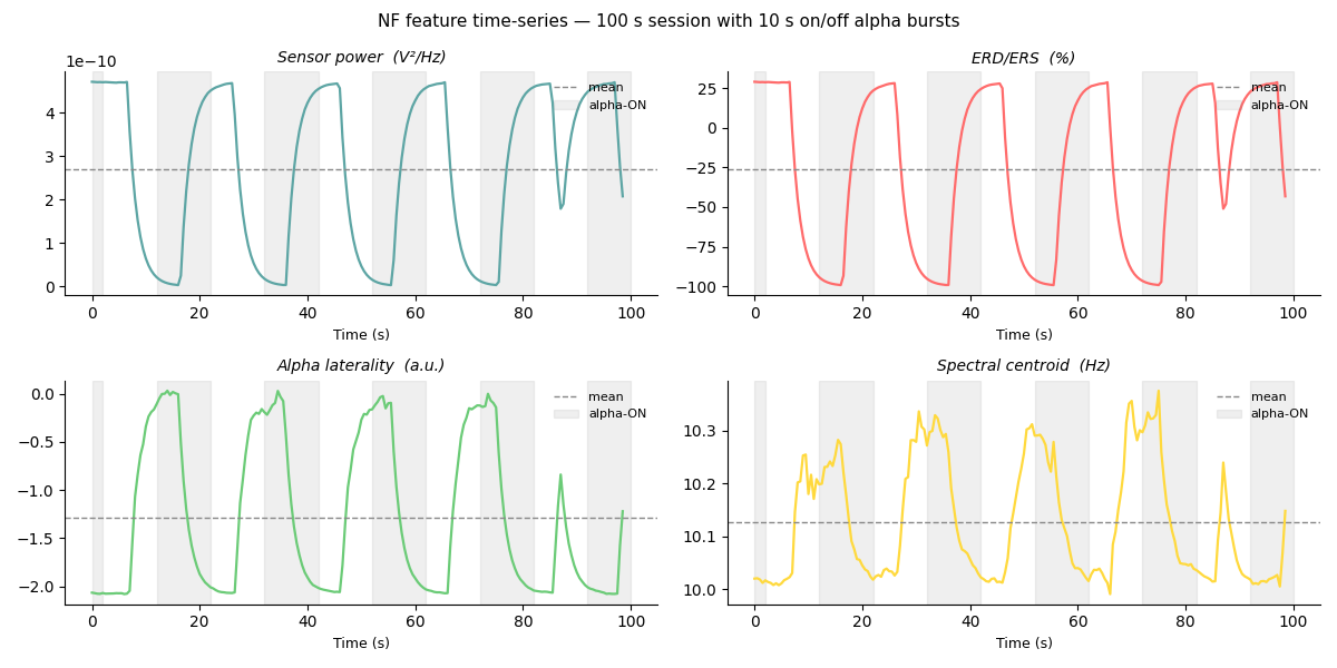
Main session started 15.8 s into the simulated file; 104 of 198 windows fall in an alpha burst.
/home/runner/work/mne-rt/mne-rt/examples/ex_complete_nf_session.py:300: UserWarning: The figure layout has changed to tight
  plt.tight_layout()